Thursday, June 30, 2022

Case-Shiller city price tiers - Low-end (cheaper) homes are riskier than high-end homes


In an earlier post we presented housing price betas for 20 large US cities using the Case-Shiller home price index. (See Case-Shiller housing price index and city price betas - Each city has a different risk profile.Home price betas will differ markedly by city. 

Case-Shiller also provides city home price data based by pricing level or tiers. Each city has three pricing tiers, low, medium, and high. This allows us to look at the appreciation in the low-end of the market as well as the high-end. One may assume that high-end homes would be subject to more risk and show greater housing betas. You would be wrong. 

Using the same methodology concerning for forming home price beta, we find that the low-end markets are often more volatile and have higher home betas.  City housing price appreciation will be correlated around tiers, but there is still significant variation.

It is noticeable that the losers from the breaking of one housing bubble may be different than the next one. Homeowners who are the most levered may be at the most risk.


Buying a low-end home is riskier than buying a high-end home. The dollars at risk may be greater for the high-end, but the return changes and drawdowns are greater for cheaper low-tier homes. The low-end buyers will be at more risk than high-end buyers if the housing market slumps from a Fed interest rate increase. 

Tuesday, June 28, 2022

Case-Shiller housing price index and city price betas - Each city has a different risk profile


The Case-Shiller housing price indices are closely followed by investors to obtain a good estimate of home price appreciation. The home price data are much richer and more detailed than just an index on a national level. Home prices can be analyzed for 20 different cities and on a national level. This is where the information gets interesting. Although there is a common element, the price appreciation for each city is different. The Las Vegas market is not the same as Detroit. A buyer of a home in San Francisco will see a different level of appreciation from a home in Boston. Hence, each city has a different return potential and risk. 

If the Fed starts to raise interest rates, it will impact home prices, but the effect will differ by city market. Some markets re more overvalued. Other markets are more stable.  A simple way to compress this information is to measure a city price index beta versus the national market. We have looked at the 20 cities available and have found there are significant city beta differences around the country. A shock to interest rates.

Using data from 2000 to the present, we have calculated the betas for 20 city markets. The West Coast cities have higher housing betas versus the Midwest. Newer cities that have seen strong demographic growth and thus have higher betas than those cities that are losing population.  


The impact of a tightening in the housing market will have a differential impact around the country. The risk of a price downturn will be greater in these high beta cities. It is worth considering the impact on region and cities from Fed policy. 

Monday, June 27, 2022

Beware, but use investor sentiment to help with hard to value stocks


Investor sentiment, defined broadly, is a belief about future cash flows and investment risks that is not justified by the facts at hand. Sentiment has a market impact on longer-term fundamentally based investors because betting against sentimental investors can be costly and risky. Smart traders and arbitragers may not be able to offset the flows from sentiment in the short run. You can call sentiment traders, noise traders that introduce volatility associated with different use of information. Hence, sentiment can cause deviations from fair value. Some stocks will be more sensitive to sentiment than others, so sentiment can be incorporated in investment decisions. See "Investor Sentiment in the Stock Market"

Sentiment measures can either be top-down or bottom-up. Given our macro focus, we will discuss some top-down conclusions. Top-down sentiment focuses on aggregated reduced form measures.  Bottom-up sentiment uses or tries to measure investor biases. Some categories of stock are more sensitive to sentiment: low capitalization, younger, unprofitable, high-volatility, non-dividend paying stocks, growth stocks and firms in financial distress. Stocks that are harder to value or more difficult to arbitrage will be subject to more sentiment risk because investors will try and use other measure to form expectations and create a perceived edge. Sentiment is associated with the propensity of marginal investors to speculate on non-fundamental information.

High (low) sentiment will push speculative stocks above (below) fair value. Easy to arbitrage or value will have less variation from fair value based on sentiment. These speculative harder to arbitrage stocks will have higher (positive) sentiment beta while more bond-like stocks will have negative sentiment betas. As information is revealed, prices should move back to fundamentals. 

What can be used for macro sentiment:

  • Investor surveys - Consumer confidence correlates with small caps and stocks with strong retail interest.
  • Investor mood - Some researchers have found a mood associated with weather and daylight.
  • Retail investor trades - Retail investors herd and can push speculative stocks.
  • Mutual fund flows - Flows are often tied to retail sentiment and will drive speculative stocks.
  • Trading value - Volume changes represent differences in opinion and especially impact stocks when short selling is difficult.
  • Dividend premium - Given more "safe" bond-like returns, there will be a premium difference.
  • Closed-end discount - The deviation from net asset value can proxy for retail sentiment.
  • Option implied volatility - Option flow trading will impact volatility and describe speculative and hedge trading.
  • IPO first-day returns - Serves as a measure of speculative fever.
  • IPO volume - Bring new firms to market is based on perceived market optimism.
  • Equity issues over total new issues - A broad measure of equity financing activity. 
  • Insider trading - A measure of what corporate insiders think about their company.

These sentiment measures can be used in concert to form a sentiment indices which can measure the deviations from fair value of speculative stocks. Sentiment can proxy for speculative demand that may be reversed as new fundamental information is released. Positive sentiment can push prices higher and create volatility only to be reversed as news enters the market.

Sentiment may not be based on fundamentals, but it can play an important role for exploiting opportunities in hard to value (arbitrage) stocks. Sentiment in other asset classes that are hard to value can be employed to measure market extremes.  


Saturday, June 25, 2022

Credit spreads and equity levels


Credit investing and equity investing are closely aligned. A bond is a put on the firm. There is only a coupon return and the return of capital. If the firm value declines, there is a decline in the value of the bond. Equity is a call option in the residual value of the firm. Both are associated with the underlying value of the company. Hence, if overall equity values increase, the risk and spread for investment and high yield should decrease. If equity markets decrease, the residual value of the firm declines and the risk to bonds will be displayed in increasing bond spreads. 

We have taken a different look at this relationship through a scatterplot with a line tracking the relationship through time. It provides a different story for how this relationship moves through time and with the level of equities.

Using data from 2012 to June 24,2022, the pandemic dominates the relationship between equites and bonds. There was a credit crisis that far exceeded the equity downturn as measured by spreads. The current equity sell-off creates a similar credit spread pattern, but it seems muted relative to the past at least for investment grade bonds. 

The more interesting relationship is the shift of the trade-off as equity levels increase. Equity markets move and then credit risk adjusts to a new level. There is not just one equity-credit spread relationship.


Credit spreads and mean reversion - works well with trends


Credit spreads for both investment grade and high yield have been increasing with the decline in equity markets. These moves have been especially strong for junk bonds with low ratings. Investment grade have seen muted performance. High yield spreads are at the highest levels in five years if we extract the pandemic liquidity crisis of March 2020. The same can be said for investment grade. Trend-trading in credit is effective especially if it is conditional on the business cycle, equity prices, and financial stability. 

Within these long-term trends, there is also opportunities for mean-reversion strategies using a z-score methodology. If spreads widen by three standard deviations, there will be a spread tightening as new money tries to take advantage of higher spreads. The same can be said for the alternative of strong negative z-scores, however, this effect is weaker since it requires as selling of gains without a natural buyer. 

Investor who are buyers of extremes and hold for even a set time will be able to capture spread mean reversion. This mean reversion can be done in conjunction with trend trading to take advantage of macro and cross-asset changes as well as market extremes. 


Fixed income factor investing - Some evidence


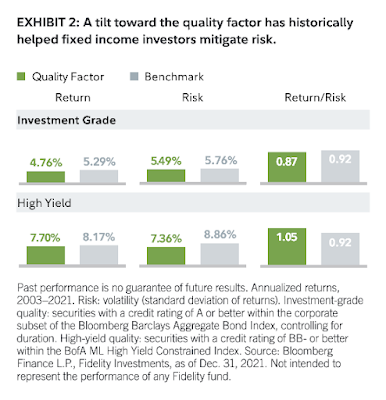
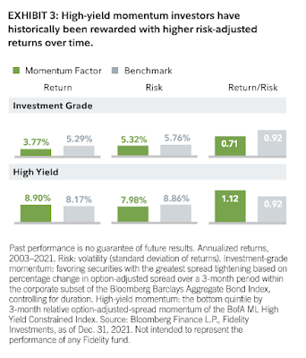
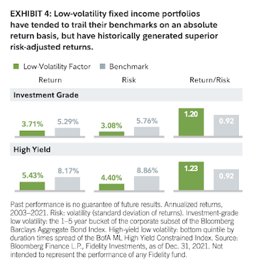
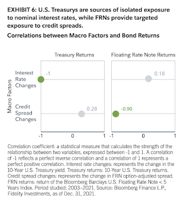
Factor investing and analysis are a normal part of equity investing; however, it has not been generally implemented within the fixed income asset class. One, good data are harder to obtain and use. Two, the relative importance versus a benchmark has not been fully analyzed. Fidelity Investments in a white paper has started to do the empirical work and have provided some key insights. Apply simple factor definitions, they find suggestive outperformance especially for high yield bonds. Nevertheless, this work only scratches the surface and needs more careful work.

Using a simple value factor based on spread cheapness associated with a rating, it is found that both investment grade and high yield increase return to risk. The returns are high, but risk is increased so the next effect is limited. 


A tilt to the quality factor shows lower returns for both investment grade and high yield; however, there is also less risk. The net effect relative to a benchmark, at least for high yield is positive. Clearly, higher quality firms, lower leverage for example, show less return and risk.


The momentum effect is strong for high yield relative to investment grade. The dispersion of spreads as well as the opportunity for upgrade are greater for high yield so there is more potential return movement for junk bonds. 


The strongest effect is for low volatility. This is the well-known effect that low duration bonds have a better return to risk. The focus of many managers is in shorter maturity sector. 


The other strong factor effect is carry. High current yield will bonds provide more return and more cushion from interest rate changes. This is the case for investment grade bonds. High yield bonds with high carry have much higher risk than a benchmark.


When isolated for the interest rate macro factors, it is found that rate changes dominate bond returns, but if isolated as a floating rate note, credit spread changes dominate returns. 


Thursday, June 23, 2022

The "two cousins" - asset and price inflation


"The real danger comes from [the Fed] encouraging or inadvertently tolerating rising inflation and its close cousin of extreme speculation and risk taking, in effect standing by while bubbles and excesses threaten financial markets." 

- Paul Volcker 

Volcker warned about the two cousins of inflation - asset and price inflation. We got the asset inflation over the last decade, but we had to wait for the price inflation after the pandemic. The asset inflation is easy to identify and control. Equities gained from strong earnings and increasing valuations. Price inflation is more complex to identify. There can be supply shocks which create relative price distortions and there can be feedback from price gains to wage increases.

The Fed is doing its job to arrest the stock market. Increasing discount rates reduces the present value of earnings and reduce the value of projects. We are in a bear market that reverses asset inflation. The price inflation has yet to be reversed. Increasing rates will reduce aggregate demand, but it is a blunt instrument. A tightening policy can reduce overall demand, but it cannot reverse gasoline prices or food prices. Weaker demand will reduce wage pressure, but it will not create new jobs. 

The Fed cannot just reduce asset or price inflation. These inflation cousins are joined together. When one goes down, the other will follow it.

The allocative effect of low rates and easy money


The negative allocative effect of low interest rates will increases as rates go higher. Simply put, the allocative effect of monetary policy is that when rates are very low for a long time (zero rate policy), investment decisions and behavior will be distorted. There are two negative effects. 

One, investors will reach for yield and invest in project that have a lower return because the risk free rate alternative is so low. For short periods, this may be a good thing for the economy, but over longer periods, investors will reach for investments that have less cushion for error. A project that has a low IRR will have a higher likelihood that the investment will lose money if something goes wrong. The margin for safety is low. 

Two, firms will have a lower acceptable return on capital. Again, the alternative is an extremely low risk free rate. As rates rise, all of these marginal projects and companies will no longer be profitable or be underwater. They were able to borrow at low rates and still have a low return on capital. Borrowing costs will increase as rates rise, but the return on capital may be the same. Defaults will increase because the slightly profitable company of yesterday will be unprofitable today and will be even less profitable tomorrow. 

I can get bad about inflation, but I worry about the negative allocative effect because that will take the economy into a recession not based on slowing aggregate demand but based on bad investments.

Wednesday, June 22, 2022

The Fed reaction function - Where all the market action is focused


Many have discussed the Fed's reaction function in the form of a simple. The Taylor Rule is the most popular of these models, yet it has fallen out of favor over the last decade; nevertheless, there still needs to be an understanding of the Fed's reaction under different scenarios. This should be the objective of forward guidance. Fed forward guidance is often obtuse and hard to unpack. What is a "soft landing"? What is "data dependent"? What is "unconditional"? 

Money is only made on trades that differ from the consensus and are correct. The Fed reaction function and trade opportunities fall into three categories: the Fed's commitment to inflation fighting, the Fed commitment to full employment, and the Fed's commitment to maintaining market stability. The Fed is unlikely to be able to manage all three in a rising rate environment. 
  • The market has discounted increases in rates, so the trade is whether Fed will become more aggressive and realize market expectations or whether the Fed will be condition in its fight against inflation. Is the Fed willing to sustain multiple 75 bps increases?
  • The market is discounting a higher probability of a recession than the Fed. If these likelihoods are true, the question is whether the Fed will again move away from its current project path of rate increases. If unemployment moves to 4.5%, will it slow rate increases or cut rates?
  • Finally, there is the question of how much financial instability will the Fed allow before acting to stem. We are in a bear market. Will the Fed be willing to see a 40+% correction and still increase rates. Will the Fed increase rates even if there was a funding problem on Wall Street. The likelihood increases as rates increase. Will the Fed sustain rate increases if there are increased threats of financial instability?
Can traders see scenarios where the Fed will abandon its inflation fighting in response to other goals. This is the big trade for 2022 and it seems likely that there are reasonable scenarios for switching priorities. Jay Powell is not Paul Volcker. The bias is toward rate increase abandonment. 

Tuesday, June 21, 2022

Investors and memory - Don't be fooled by only focusing on the good trades


You have heard this story. I am a good investor! Why? Because I have a good memory of my past trades and those trades have all worked out. This is a nice narrative, but it is not true. Some recent researchers formed some structured experiments and found that most investors have a memory bias. (See "Investor Memory".) 

The researchers tested for a memory effect or bias with investments. They found that subjects over-remember positive outcomes and under-remember negative returns. This pattern of remembering leads to overly optimistic beliefs and reinvestment. Any bad trades will soon be forgotten while those winners will be front and center in an investor's mind. It takes a special investor to focus memory on both good and bad decisions.  

Other researchers have found that positive memory biases lead to overconfidence and more trading. If I think I am right, I should do more of the same. (See "Investor memory of past performance is positively biased and predicts overconfidence") However, by exposing investors to their bad trades and training them not to have a positive bias, this overconfidence and memory bias can be reduced.

A quantitative model will not have a memory bias. It will view positive and negative decisions the same. There is no extra training needed, no overconfidence, no belief bias, and no excessive trading. If you don't use a model, at least spend time reviewing bad trades to minimize a memory bias.

Monday, June 20, 2022

Credit drives all financial and real markets


Let's be clear. Credit or more precisely the cost of credit drives all markets, financial and real. If there is a repricing of credit, that is a rise in rates, it will affect all markets in a significant number of ways. This repricing occurs even if inflation is higher than nominal rates because inflation impact firms differently.  

  • Increase in the risk-free rate of return will reverse the reach for yield when rates were close to zero.
  • An increase in the discount rate will reduce the present value of all cash flows. Firms that expect more distant cash flows will be more affected.
  • Rising rates will reduce cash available for investors and projects if rates go higher; more will go to debt holders.
  • The cost of capital will increase, so investment projects will be rejected.
  • Firms that made a low return on capital but above zero were able to continue operations. It will be the case as rates increase. Firms will go out of business. 
Financial markets begin and end with what is happening in credit markets, so repricing of credit will fundamentally change not just debt markets but the pricing of equities and the success of firms which spills into the real economy. A credit crisis will create an equity and real economy crisis.


Sunday, June 19, 2022

Central banks and being behind the curve this week


There is the old joke about wearing running shoes in the woods as a protection against bears. All you need to do is outrun the other hikers not the bear. The dollar is appreciating because Fed monetary policy is outrunning other central banks at being more hawkish. It is showing in currency pairs. The only exception with tightening is the BOJ which is holding to its loose policy. All central banks are acting as though they are behind the inflation shock. All these banks are giving forward guidance that rate increases will increase. 

  • Fed raise 75 bps forward guidance more tightening 
  • SNB raises 50 bps forward guidance more tightening
  • BOE raises 25 bps forward guidance more tightening 
  • Brazil raises 50 bps 
  • BOJ holds policy forward guidance more of the same 
The global tightening is clearly signaling that risk assets should be repriced around the globe. Tracking country trends using short, intermediate, and long-term models, we find that all are giving a short signal. The only exception is China which is coming out of their aggressive lockdown and showing some improvement in macro numbers. When there was central bank commonality with adding liquidity, equity market moved higher. Now we are seeing a major reversal in both equity and fixed income markets. Call this the Great Risk Repricing Crisis.


Friday, June 17, 2022

Bear markets and recession - A serious signal


The eminent economist Paul Samuelson famously quipped that the stock market had predicted nine of the past five recessions. The numbers above suggest something different but realize that you must be careful about how the term "bear market" is defined. If you look at other indices, you may get different results. 

Nevertheless, the combination of a stock market bear and an inverted yield curve is a good combination of recession signals. The bear market could be a repricing of market risk, but it also can be a signal about future earnings that are driven by the real economy. We are repricing equity values given higher inflation and higher yields. 

That factor combination does not mean we will have a recession; however, tighter money conditions with a more difficult environment for pricing costs and output is a recipe for a recession. We certainly are in a stagflation environment.

Monday, June 13, 2022

Consumer sentiment index shows strong pessimism


The University of Michigan consumer sentiment number at 50.2 is at the lowest levels ever recorded. The last time we were this low was in 1980 when we were feeling the worst effects of the inflation, oil shock, and Fed tightening at the end of the Carter Administration. The only time we get these low numbers are when we are entering a recession. 

What is as disturbing is the acceleration of the decline. Of course, we are seeing an oil shock, an economic slowdown, and rising interest rates, yet the job situation is still positive, household balance sheets are in good shape, and housing, the sector where most wealth is held, is firm. This is all about the pump and the shopping basket; however, it still matters and can feed on itself. 

The Fed now has the dual problem of solving inflation while not driving the economy into a recession. This is much worse than expected because inflation is closely tied to a supply shock that cannot be easily addressed through monetary policy.

Inflation - More volatile and stronger short-term moves

The CPI announcement was higher than expected for the headline number at 8.6% versus 8.3% and core was at 6% versus 5.9%. The big surprise was the headline MOM which increased 1% versus .7%. There is a clear increase in inflation volatility. Volatility of 12-month changes is at the highest levels since the GFC when we had outliers on the downside. More interesting, the core volatility is increasing and closing the gap with headline inflation. Core inflation is usually more stable than the headline numbers. Volatility will increase with the level of inflation. The volatility increase in the core inflation is disturbing. 

If volatility increases, there should be a decline in the sensitivity of a small change in inflation. That was not the case for Friday's number. Inflation has become the focus of investors and any change will have a heightened response. We are expecting 70s and 80s type of inflation responses and not the limited response over the last 10 years. 


Thursday, June 9, 2022

How persistent or transitory is inflation?


Inflation is volatile based on monthly changes. The variation away from an average monthly equivalent will be large with most of the negative spikes since 2000. The current monthly PCE changes are persistent and getting larger. The recent higher trend takes us back to a 2% trend for the last ten years. The PCE price index grew only 1.38% from January 2012 to February 2020. The last two years have seen a growth rate of 4.2%. 


The researchers at the San Francisco Fed have looked at the persistence of inflation levels and changes. See "Untangling Persistent versus Transitory Shocks to Inflation". Both are moving higher after a period of low correlation. This information can be used to describe transitory and persistent inflation. Transitory inflation is a shock away from a longer-run value with a shift in the longer-run value over time. A persistent shock is one that shifts the longer-run value. This can be seen through the correlations of levels and changes. A high correlation of inflation levels shows persistence. A high correlation with inflation changes, less negative, shows that transitory inflation is low. 

A shock volatility is the ratio of level and change persistence. The shock volatility ratio is the standard deviation of persistent shocks divided by the standard deviation of transitory shocks. A level above one says that persistence shocks are more volatile than transitory shocks. We saw high levels in the last decade, but the overall inflation was low. We are now seeing persistence at higher inflation levels. 


Wednesday, June 8, 2022

Sector classification is a dynamic process


Classification is static in most sciences. An animal or plant is classified and unless there are some clear mistakes in identifying the species, it will maintain its classification. New species will be added as discovered but there will not be switching. Of course, we have some significant counterexamples like the controversy as to whether Pluto is a planet. 

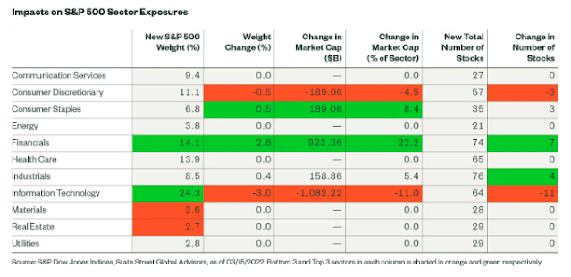
In the case of financial indices, there are dynamic adjustments based on the changing nature of businesses and firms. S&P released classification changes this spring to be implemented in 2023. Below is a list of the new classifications and the impact on S&P 500 sector exposures. There is enough time for firms to adjust, but it is important to realize that classifications are man-made constructs and not a function of some statistical properties.

Correlation differences within an industry may have everything to classification and not opportunities for trading pairs of securities. 


Commodity super-cycle is here but different from the past


A simple chart from our friend, Tom Pickering at Auspice, describes the foundation for this current super-cycle. Commodity super-cycles do not follow the credit or business cycle although both these cycles can support and reinforce the commodity super-cycle. 

A commodity super-cycle has three key drivers. An unexpected and sustained increase in demand. A shortfall in past investments that reduces new supply. Short-term catalysts that cause price spikes and leads to logistical disruptions. 

The demand issue is associated with the pandemic; however, this shock is not the same as the increase in China commodity demand which was the cause of the last super-cycle. Underinvestment is curtailing supply. A lack of capital will be a major catalyst for the super-cycle. The underinvestment problem is threefold. One, a lack of investment in some commodity sectors have a long-term effect that only shows itself when there is a market shock. Two, there is greater need for mining investment to account for the renewable and EV revolution. This is a relative investment issue but will drive key markets. Three, there is the underinvestment caused by the switch to ESG investing. Commodity extraction is a dirty business and has been avoided.  

The catalysts for the current price shocks are the pandemic and Ukraine War which has stressed logistics and has created a rethinking of where and how commodities are sourced and transported. The government policies through regulation and sanction. creates a new costly environment. These catalysts create a reordering of investments which was unexpected. Commodity logistics cannot be easily changed in the short run.

The easy money may have already been made in commodities, but the overall opportunities in this sector will continue. Super-cycles can last for years, and the current backwardation is favorable for long investors.  
 

Tuesday, June 7, 2022

Know the counter-argument for any investment


“He who knows only his own side of the case, knows little of that.” 

— John Stuart Mill 

"I never allow myself to have an opinion on anything that I don’t know the other side’s argument better than they do." 

- Charlie Munger 

"Ignorance more frequently begets confidence than does knowledge."

- Charles Darwin

If you want to understand your position in any argument, learn what is the counter-argument. Whether associated with investing or current events, serious knowledge of the alternative will only help you refine your position. Describing pros and cons of any investment is a critical skill, yet it is harder than most think. Of course, it is easy to detail the arguments that support a position, and then the counter-arguments become a perfunctory process with minimum effort. A counter-argument cannot be the mirror opposite of an existing position, nor can it be a straw man that can be easily defeated. A good counter-argument should have the potential to be persuasive.

For example, someone could argue that the Fed is going to follow a hawkish policy because inflation is going higher given continued supply congestion and oil price increases. The counter-argument cannot just be that oil prices and bottlenecks will be reversed. The process of why must be detailed and given specificity. 

The counterargument issue becomes especially difficult when developing quant models. There is no counterargument except through breaking the model, running alternative scenarios, or having another model to contrast against the primary model. There is a reason for why ensemble modeling is used to solve the counterargument problem. What do alternative models say about output?


Monday, June 6, 2022

The Global Supply Chain Pressure Index worth following


The New York Fed Global Supply Chain Pressure Index (GSCPI) is a good way to look at the driver that affect supply pressure shocks on inflation. The numbers exploded after the pandemic began and got worse during the second COVID wave and is still at high levels versus spring of 2020. The numbers have come off the 4 standard deviation peaks, but there the decline has now plateaued. For more details see the NY Fed May 2022 paper #1017 "The GSCPI: A New Barometer of Global Supply Chain Pressures"

The following graphs provide insights on the areas which have had the greatest impact on the recent GSCPI. The China lockdown is having a global effect. The color graphs show the impact of supply chain, oil supply, and oil demand on US PPI and CPI and Euro area PPI and CPI. Oil supply and demand have had a more variable impact on inflation, but supply chain price pressures have been consistent over the last two years.

The bottom-line is that if this global supply chain index declines, we will see an appreciable impact on the PPI and CPI indices.


Davos and globalization


The researchers at the World Economic Forum (WEF), Davos, presented a white paper on globalization that is worth thinking about. It divides the future of globalization into four scenarios based on a two-by-two matrix of physical and virtual fragmentation or integration. Global connections can be through either through physical trade or some form of virtual or non-physical trade which represent high tech integration. (See "Four Futures for Economic Globalization: Scenarios and their Implications" White Paper May 2022 WEF.) I prefer a physical versus services trade matrix with a third dimension associated with finance, but we can use the WEF for discussion.

The physical trade world is clearly disrupted on two dimensions. Supply chain problems from the pandemic have altered how firms and countries view logistics and where they are sourcing goods. The Ukraine War has created a new view that each country must think about self-sufficient with respect to key physical goods like food and energy. The virtual globe world is changing rapidly as countries attempt to control the flow of data and communication. 

Scenario 1 represents the old world of globalization prior to the pandemic. It may be the desire for many to move back to this world, yet it is less likely given the shock events of pandemic and war. Even the virtual world may see less integration although it many have switched from physical contact to virtual communication. Physical integration may occur albeit less concentrated with fragmentation of e-commerce and communication. The reverse of physical fragmentation and virtual integration is the opposite choice with selection to bring manufacturing home but outsource some intellectual activities for cost benefit. 

Nevertheless, the great fear is a movement to isolation around the world as nations attempt to protection commodity sourcing and onshore more activities. The US has started to discuss the idea of friend shoring where countries pick their trading partners as a way of protecting national interests. This will be the great fear to the liberal order of free trade and will have strong implications for firms trying to navigate cost minimization.

The bottom-line for investors is that country financial markets will become delinked and reduce correlation. International diversification will increase but there will be greater dispersion in returns and more room for active investing. Nonetheless, the focus will change from picking firms to picking countries based on strategic partnerships across governments.  

Data and lawlessness - think in frequency and when in doubt, think random


In his well-written book, Chancing It - The laws of chance and how they can work for you, Robert Matthews explains well the basics laws of chance and probability, but he also spends time describing what he calls the principles of lawlessness. It is a nice device to remember some important statistical concepts. 

The first law of lawlessness - do not look at events look at the frequency of events. Every number should be looked at in context, the context of likelihood. Ask the simple question - what is normal and what is abnormal. Risk management is all about getting the frequency right. 

The second law of lawlessness - When trying to understand random events don't assume they are independent and don't assume that correlated events will stay that way. Live would be so simple if the events were independent. The probability of A and B occurring is just the product of the individual probabilities. However, if you know the correlation of two variables, do not assume that this correlation will stay the same. Correlations change and may be related to a third variable.

The third law of lawlessness - randomness does not ultimately have patterns; but in the short-run there can be regularity. When in doubt, go with random. You may think you see a pattern in the short run, but that does not mean the pattern will continue, nor does it say that a time series is non-random. A random series does not mean-revert. A series of heads does not mean the next flip is more likely a tail, yet in the long run the frequency of a tail is .5.

Be cautious of any number and any count. A small sample will tell a different story from a large sample and the actual likelihood may be different from any data collected. When in doubt, trust randomness. 


Sunday, June 5, 2022

The fiscal policy bet that led to more inflation


US inflation is higher than other countries in the OECD. The difference is significant and started last year before the Ukraine War. We have been running the economy hot even before the pandemic based on relative inflation. We are now seeing he results of these policies. 
Charts are from a good short research piece from the San Francisco Fed, "Why is US inflation higher than in other countries?" 

At the same time, the real disposable income has jumped to higher levels than other OECD countries. Disposable income was similar to other OECD countries before the pandemic. US fiscal policy pushed disposable income higher versus the rest of the developed world. The fiscal policy spikes are now normalizing. 

If the fiscal support was not present inflation in the US would be 3 percent lower than current levels which would put the US back in the OECD range. The US made a bet to aggressively expand fiscal policy to maintain the real economy during the pandemic. It may have been assumed that inflation would be higher given this stimulus, but since the US was just below the 2% target, the Fed and US government were willing to accept the risk. The oil and logistic supply shocks as well as the war were not fully expected. It was a policy bet and it has not worked out with respect to inflation. It should be owned, but the investment question is what will now happen.

First, monetary policy is becoming restrictive. The Fed may be moving faster than other central banks, for example, the ECB.  Second, there is no BBB bill that is pending or has been approved so the fiscal policy has become more restrictive and consistent with other countries. Hence, we should see inflation move back to OECD averages. Inflation should normalize at a level lower than current headlines. What is unclear is the timing. It is easy to argue for inflation mean reversion, yet it may not come until the end of the year and that will be at the price of lower aggregate demand.